Text Mining The Hobbit · Fisher Ankney

After recently finishing J.R.R. Tolkien’s The Hobbit, I wanted to dive further into Tolkien’s world by trying my hand at text mining the book in R. Without any previous text mining experience or goals for the project, I decided to do what any reasonable person would do and I looked to the internet for help. After reading a text mining with R e-book, this R-Bloggers Metallica lyric analysis post, and this Data Camp text mining blog post, I had some idea of what I wanted to do. I think in the end the analysis went well enough, if not a little bit long, but you be the judge.

This text project is broken into three parts – a traditional word frequency analysis, a character analysis, and a sentiment analysis. Here is the copy of the hobbit that I’m using if you want to follow along. Without further ado – here’s hobbits.

Load Libraries

library('tidyverse')    # used for EVERYTHING
library('stringr')      # used for string (text) manipulation
library('tidytext')     # used for text mining
library('wordcloud')    # used for creating cool text visualizations

Load Data

the_hobbit <- as.tibble(read_file("input/hobbit_body.txt"))

Tidy Data

tidy_hobbit <- the_hobbit %>%      # copy the_hobbit text into tidy_hobbit
  unnest_tokens(word, value) %>%   # each word is given a cell in tibble
  anti_join(stop_words)            # take out meaningless words like a, to, and it

View Data

head(the_hobbit)

## # A tibble: 1 x 1
##   value                                                                   
##   <chr>                                                                   
## 1 "Chapter I \r\rAN UNEXPECTED PARTY \r\rIn a hole in the ground there li…

head(tidy_hobbit)

## # A tibble: 6 x 1
##   word      
##   <chr>     
## 1 chapter   
## 2 unexpected
## 3 party     
## 4 hole      
## 5 ground    
## 6 lived

A quick note: I cleaned up the hobbit text to start at Chapter 1 and end the finish of the last chapter before I saved it as an input file. head(the_hobbit) reveals a 1x1 table with the entire novel stored as a single string in the tibble. This formatting has some uses so I’ll keep a copy of it, but the transformed text, tidy_hobbit is even more useful.

tidy_hobbit has cut out some words - in, a, in, the, there, and so on. That’s the anti_join(stop_words) at work. anti_join( ) is a dplyr function loaded from the tidyverse, it’s job is to return all rows from x where there are not matching values in y. In this case x is the_hobbit, y is stop_words, a tibble from the tidytext library. Also notice that now each word has it’s own row in the tibble, pretty tidy.

Word Frequency

How many words are in The Hobbit?

str_count(the_hobbit, " ") + 1

## [1] 95874

How many sentences?

str_count(the_hobbit, "[.!?]")

## [1] 5967

How long should the book take to read?

((str_count(the_hobbit, " ") + 1) / 200) / 60 # number of words / 200 words-per-minute / 60 minutes

## [1] 7.9895

Frequency Plot

What are the most common meaningful words in The Hobbit? To find out, let’s create a frequency plot. These graphs that illustrate counts of various categories are some of my favorite to create.

tidy_hobbit %>%
  count(word, sort = TRUE) %>%          # count words
  filter(n > 80) %>%                    # only show words that have been used 80+ times
  mutate(word = reorder(word, n)) %>%   # sorts words by decending occurance
  ggplot(aes(word, n)) +                # plot the words vs number of occurances
    geom_col(fill = "darkslateblue") +  # blue bars
  xlab("Word") +                        # labels
  ylab("Number of Occurances") + 
  labs(title = "Most Common Meaningful Words in 'The Hobbit'") +
  coord_flip() +                        # sideways box-plot for aestetic purposes
  theme_minimal()                     

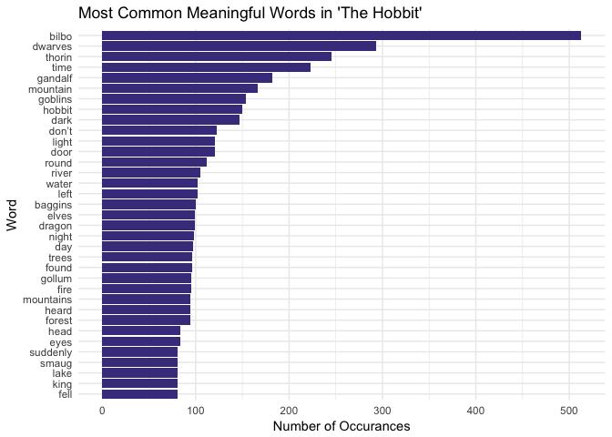
The most common words in The Hobbit are Bilbo, dwarves, Thorin, time, and Gandalf. The only non-character word is time, but I bet the word time is common enough in most novels. I’m surprised to see the word “don’t” on the list, I thought it was classified as a stop word. There isn’t much to be surprised about on this list if you’ve read the book, and If you haven’t read the book, the list gives you a pretty good idea of what to expect!

Now this plot is pretty cool and informative, but can we make it more artsy?

Word Cloud

hobbit_cloud <- tidy_hobbit %>%
  count(word) %>%                                      # provide a count of each word
  with(wordcloud(word, n, max.words = 100,             # using the wordcloud library, plot word, according to n (number of count), with 100 maximum words)
                 color = brewer.pal(n = 8,"Set1")))    # use RColorBrwer pallete 'Set1'

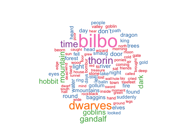
Here’s the more artsy (and less informative) word cloud! These are the top 100 words used in The Hobbit. I’m not sure what’s with the color coding, but the size of the word is dependent on its number of appearances in the book.

Character Analysis

Now let’s dig into the main characters of the novel. Who are the most important characters and where do they appear most in the book?

Main Character Count

main_chr <- as.tibble(c("bilbo", "thorin", "gandalf", "smaug", "gollum", "bard")) %>%
  unnest_tokens(word, value)      # defining the main characers

colnames(main_chr) <- "word"      # naming the column of characters

main_chr_num <- tidy_hobbit %>%   # moving tidy_hobbit to a new var
  semi_join(main_chr, "word") %>% # only keep tidy_hobbit lines that have main_chr
  count(word, sort = TRUE) %>%          # count presence of each character
  mutate(word = reorder(word, n)) %>%   # reorder characters by number of occurance
  ggplot(aes(word, n)) +                # plot the results
    geom_col(fill = "darkslateblue") + 
    labs(title = "Main Characters in 'The Hobbit'") + 
    xlab("Character") + 
    ylab("Count")
main_chr_num

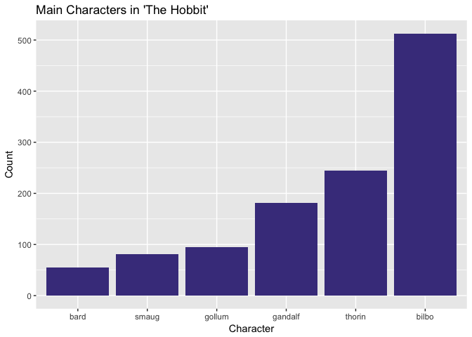
As we saw in the word frequency plot, Bilbo is not only the most important character out of the six I’ve listed, but his name is the most common word in the entire book. Life is good being the protagonist! Thorin the dwarf king is mentioned some 250 times, and Gandalf is mentioned under 200 times. I would have thought Gandalf played a bigger role than Thorin, but I guess the counts don’t lie. Gollum, Smaug, and Bard are comparatively minor characters.

tidy_hobbit$linenumber <- 1:nrow(tidy_hobbit)  # label 'linenumbers'

main_chr_pres <- tidy_hobbit %>%       
  semi_join(main_chr, "word") %>%       # keep only the six main characters in the hobbit text
  ggplot() + 
  geom_point(
    aes(word, linenumber)              # plot character name and linenumber they appear in
  ) + 
  labs(title = "Main Character Apperances in 'The Hobbit'") +
  xlab("Character") + 
  ylab("")+
  coord_flip() + 
  theme_minimal() + 
  theme(axis.title.x=element_blank(),
        axis.text.x=element_blank(),
        axis.ticks.x=element_blank())
main_chr_pres

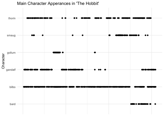
By the looks of it, Bilbo is basically mentioned every other sentence. There are two small gaps in Bilbo’s presence near the end of the book where Bard takes the center stage for a bit. Devilish ol’ Smaug is briefly mentioned in the first half of the book, something along the lines of “oh, there’s also a dragon guarding the gold but don’t worry about it until later”. Gandalf makes three dramatic apperances throughout the tale, he does an interesting timeline, he has three solid appearances in the tale, sitting out for the stories climatic Smaug-burglary.

Dwarf Character Count

dwarf_chr <- as.tibble(c("dwalin", "balin", "kili", "fili", "dori", "nori", "ori", "oin", "gloin", "bifur", "bofur", "bombur", "thorin")) %>%                      # a list of the 13 dwarves
  unnest_tokens(word, value)   

colnames(main_chr) <- "word"        # label the values column "word"

dwarf_chr_num <- tidy_hobbit %>%   
  semi_join(dwarf_chr, "word") %>%  # keep only the dwarves names from the main text
  count(word, sort = TRUE) %>%      # sort the dwarves by apperance count
  mutate(word = reorder(word, n)) %>%
  ggplot(aes(word, n)) + 
    geom_col(fill = "darkslateblue") + 
    labs(title = "Dwarves in 'The Hobbit'") + 
    xlab("Dwarf") + 
    ylab("Count")
dwarf_chr_num

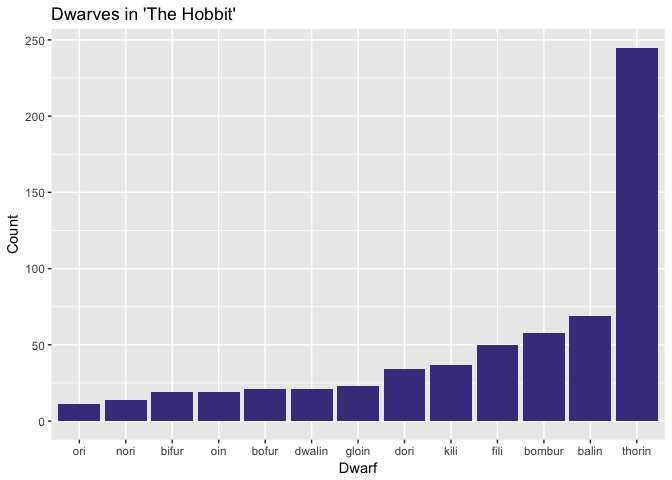
Poor Ori is only mentioned about a dozen times. Ori, Nori, Bifur, Oin, Bofur, Dwalin and Gloin are really nothing but background characters. Fili is mentioned a bit more than his twin Kili. Bombur, the rotund comic relief dwarf is actually a fairly important character Balin is much more important than his younger brother Dwalin, which makes sense because Balin is the second eldest of the bunch and often the leader in Thorin’s absence.

dwarf_chr_pres <- tidy_hobbit %>% 
  semi_join(dwarf_chr, "word") %>%
  ggplot() + 
  geom_point(
    aes(word, linenumber)
  ) + 
  labs(title = "Dwarf Apperances in 'The Hobbit'") +
  xlab("Dwarf") + 
  coord_flip() + 
  theme_minimal() + 
  theme(axis.title.x=element_blank(),
        axis.text.x=element_blank(),
        axis.ticks.x=element_blank())
dwarf_chr_pres

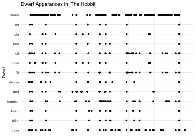
The dwarves sure are a tribal bunch; if Tolkien mentions one of the background dwarves he almost always mentions the rest of them in the next breath. It’s hard to tell that Fili is a little bit more important than his twin Kili from this plot. Balin and Thorin’s only noticeable absence is when Bilbo finds the ring and bests Gollum in a battle of wits.

Word Sentiment

Using the tidy text package we can analyze word sentiment throughout the tale. I use two types of sentiment measurements in this analysis. Descriptive “NRC” package sentiment counts words that express an emotion, such as anger. Cumulative “AFINN” package sentiment is an overarching positive / negative word summation. There’s a third type of sentiment library in tidytext, but I forget it’s name right now.

Joyous Sentiment

nrcjoy <- get_sentiments("nrc") %>%    # using the nrc sentiment package in the tidy text library
  filter(sentiment == "joy")           # using only words that have a sentiment of joy

happy_cloud <- tidy_hobbit %>%         # put the tidy_hobbit into a new variable
  inner_join(nrcjoy) %>%               # only keep words that match the nrcjoy variable 
  count(word) %>%                      # now count the number of times each word is used
  with(wordcloud(word, n, max.words = 100,  # create a word cloud based on this
                 color = brewer.pal(n = 8,"Dark2")))

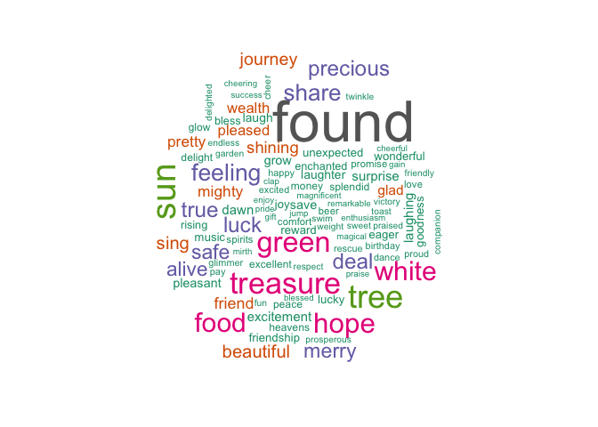
These are the top 100 words Tolkien uses to describe joy in The Hobbit! I think this is the coolest visualization so far. So many of these adjectives just encompass the adventurous comradery present in the book.

joy_meter <- tidy_hobbit %>% 
  inner_join(get_sentiments("nrc")) %>%  # same as above
  filter(sentiment == "joy") %>%
  group_by(index = linenumber %/% 500) %>%  # group joy count by every 500 words
  summarise(sentiment = n()) %>%  # sentiment = number of joy words (per 500 words) 
  mutate(method = "NRC")          # call NRC method from tidy text

joy_meter %>%                     # plot results
  ggplot(aes(index, sentiment)) +
  geom_col(show.legend = FALSE,
           fill = "orange") + 
  xlab("Book Progression") + 
  ylab("Joy Meter") + 
  labs(title = "Words with Joyous Sentiment in 'The Hobbit'") +
  theme_minimal()

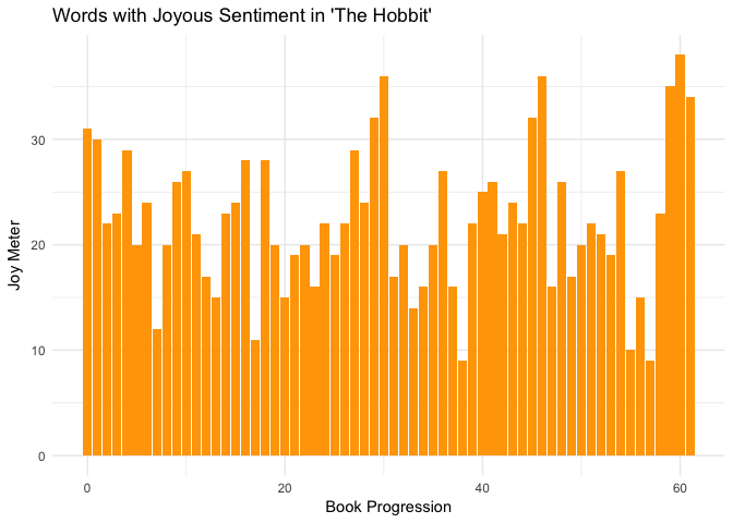
This is a plot of words that express joy as they appear throughout the book. Each index is 500 meaningful words, so the first bar of the plot tells us that 31 of the first 500 meaningful (non-stop word) words in The Hobbit express joy.

Sad Sentiment

nrcsad <- get_sentiments("nrc") %>%    # from the tidytext
  filter(sentiment == "sadness")

sad_cloud <- tidy_hobbit %>%
  inner_join(nrcsad) %>%
  count(word) %>%
  with(wordcloud(word, n, max.words = 100,
                 color = brewer.pal(n = 8,"Dark2")))

sad_meter <- tidy_hobbit %>% 
  inner_join(get_sentiments("nrc")) %>% 
  filter(sentiment == "sadness") %>%
  group_by(index = linenumber %/% 500) %>% 
  summarise(sentiment = n()) %>% 
  mutate(method = "NRC")

sad_meter %>%
  ggplot(aes(index, sentiment)) +
  geom_col(show.legend = FALSE, 
           fill = "lightsteelblue") + 
  xlab("Book Progression") + 
  ylab("Sad Meter") + 
  labs(title = "Words with Sad Sentiment in 'The Hobbit'") +
  theme_minimal() 

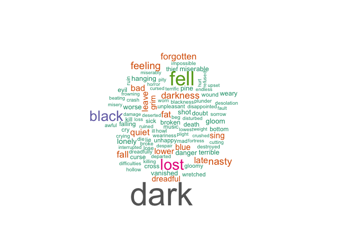
The sad sentiment meter is much higher than the joy sentiment meter, which is strange because I came away from The Hobbit thinking it was a happy book. The sad words in the word cloud are a bit generic, let’s try analyzing fear throughout the book.

Fearful Sentiment

nrcfear <- get_sentiments("nrc") %>%   
  filter(sentiment == "fear")

fear_cloud <- tidy_hobbit %>%
  inner_join(nrcfear) %>%
  count(word) %>%
  with(wordcloud(word, n, max.words = 100,
                 color = brewer.pal(n = 8,"Dark2")))

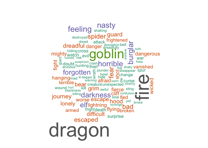
Now this is a good word cloud! Dragon, goblin, fire, escaped, darkness, spider! This visualization really gives you a feel for all of the dreadful things Bilbo and the dwarves endured on their quest for treasure.

fear_meter <- tidy_hobbit %>% 
  inner_join(get_sentiments("nrc")) %>% 
  filter(sentiment == "fear") %>%
  group_by(index = linenumber %/% 500) %>% 
  summarise(sentiment = n()) %>% 
  mutate(method = "NRC")

fear_meter %>%
  ggplot(aes(index, sentiment)) +
  geom_col(show.legend = FALSE, 
           fill = "Red4") + 
  xlab("Book Progression") + 
  ylab("Fear Meter") + 
  labs(title = "Words with Fear Sentiment in 'The Hobbit'") +
  theme_minimal()

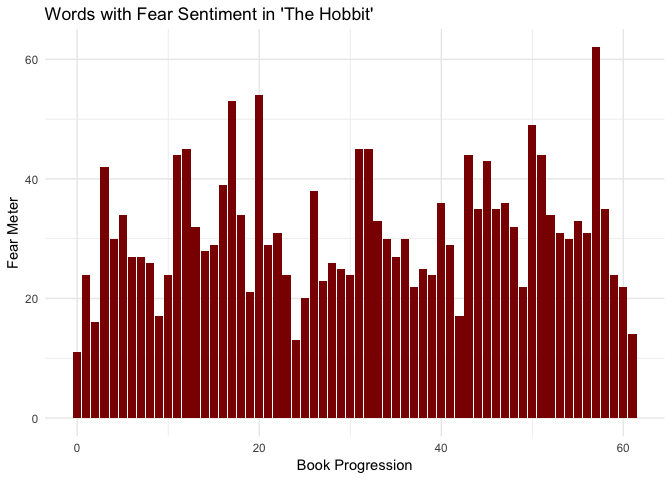
Also pretty high fear counts. Let’s see how fear, sadness, and joy stack up against each other throughout the book.

All Together Now

ggplot() + 
  geom_smooth(aes(fear_meter$index,
                  fear_meter$sentiment, 
                  color = "Fear"),
              se = FALSE) + 
  geom_smooth(aes(joy_meter$index, 
                  joy_meter$sentiment, 
                  color = "Joy"),
              se = FALSE) + 
  geom_smooth(aes(sad_meter$index, 
                  sad_meter$sentiment, 
                  color = "Sadness"),
              se = FALSE) + 
  xlab("Book Progression Index") + 
  ylab("Sentiment Index") +
  labs(
    title = "Specific Sentiment in 'The Hobbit'"
  ) + 
  theme_minimal() + 
  scale_color_manual(
    name = "Sentiment",
    values = c("red4", "orange", "lightsteelblue")
  )

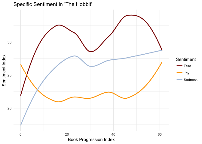
Just as I gathered from the individual meters, The Hobbit starts off cheerful enough but then becomes 300 pages of fear and sadness before a brief respite in the last chapter or two. But it’s hard to be convienced, The Hobbit didn’t feel like a scary or dreadful book! Let’s try analyzing this with the AFINN sentiment analysis method.

AFINN Sentiment

hobbit_sent <- tidy_hobbit %>% 
  inner_join(get_sentiments("afinn")) %>% 
  group_by(index = linenumber %/% 500) %>% 
  summarise(sentiment = sum(score)) %>% 
  mutate(method = "AFINN")

hobbit_sent[["sign"]] = ifelse(hobbit_sent[["sentiment"]] >=0, "positive", "negative")     # Creating a sign variable based on positive or negative sentiment

hobbit_sent %>%
  ggplot() + 
  geom_col(aes(index, 
               sentiment,
               fill = sign)
           ) + 
  scale_fill_manual(name = "Sentiment",
                    values = c("positive" = "royalblue4", "negative" = "red4"),  # turning negative sentiment red, positive blue
                    guide = guide_legend(reverse=TRUE)) + 
  xlab("Book Progression Index") + 
  ylab("Sentiment Index") + 
  ggtitle("General AFINN Method Sentiment in 'The Hobbit'") + 
  theme_minimal()

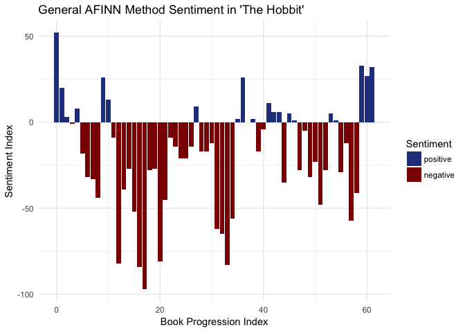
Well I guess that settles it, J.R.R. Tolkien’s fantasy novel plainly a downer. Don’t read The Hobbit if you’re looking for a pick me up! I guess if anything these results can be used to help build the case for the power of compliment sandwiches and the like.

There’s a lot more you can do with text analysis, but I think this is a good stopping point for me. Text mining The Hobbit has actually been a really fun project, it made me follow the rabbit-hole of text mining further than I originally thought I would.

There are many packages and methods for text mining, tidytext is just the one I happened to stumble upon. Some say that over 70% of the data created every day isn’t nice rectangular datasets, but data embedded in maps and papers and other sub-optimal mediums. Maybe with the right text analysis tools and skills skill set, .pdf’s don’t have to be the place that data goes to die.

I hope you enjoyed following my own adventure in the realm of text mining!

Until next time,

- Fisher