Introduction
This is the fourth of eight installments of my Unpacking the Tidyverse series. Each installment focuses on one of the eight core packages in Hadley Wickham’s tidyverse. Instructions given in each post are mainly derived from Hadley’s textbook, R for Data Science, and CRAN package documentation. This installment of Unpacking the Tidyverse focuses on the data-tidying package, tidyr. The previous installment focuses on the dplyr package, and can be found here. The next installment focuses on the tibble package, and can be found here.
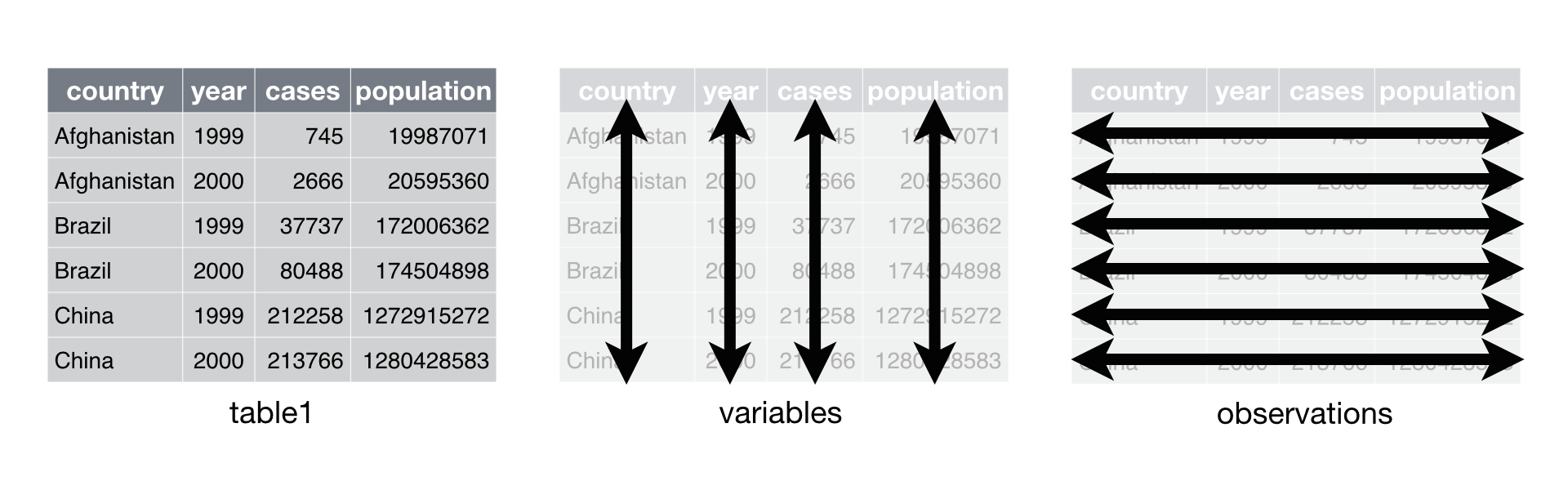
Tidy data is an easy and consistent way of storing data that makes future analytical steps simpler. Datasets that follow the three tidy data rules allow for R’s vectorized nature to work its magic. The package tidyr is meant to coerce your dataset to follow the three rules of tidy data; it is not meant for general reshaping or aggregating of data.
Tidy Data Rules:
- Each column is a variable
- Each row is an observation
- Each value has its own cell
library('tidyverse')
Important Package Functions
gather()        # Takes multiple columns and collapses into key-value pairs
spread()        # Spreads a key-value pair across multiple columns
separate()      # Single column into multiple columns, defined separator
unite()         # Multiple columns into single column, defined separator
complete()      # Turns implicit missing values explicit
fill()          # Fills in missing rows in a column based on the last entry
gather()
Often, a dataset has column names that are not the names of variables,
but the values of variables. take table4a for example.
table4a

## # A tibble: 3 x 3
##   country     `1999` `2000`
## * <chr>        <int>  <int>
## 1 Afghanistan    745   2666
## 2 Brazil       37737  80488
## 3 China       212258 213766
In table4a, the column names 1999 and 2000 are values of the
variable year, not variables themselves. The gather() function can fix
this, it is perhaps the most commonly used function in tidyr. Begin by
listing the column names that are actually variable names into
gather() as its first arguments. Once these column names have been
entered, define a key as the second argument. In this case, 1999 and
2000 are both years, so the key, or new variable name, is year.
Finally, define a value to be associated with the key as the last
argument in gather(). The value is the name given to the elements
that were previously linked to the previous 1999 and 2000 false
variables. Because these two years have been gathered into a new year
variable, the associated elements need a new column to call home. In
this case, the values represent a number positive cases, so the value
is now defined as cases.
table4a %>%
  gather(`1999`, `2000`, key = "year", value = "cases")

## # A tibble: 6 x 3
##   country     year   cases
##   <chr>       <chr>  <int>
## 1 Afghanistan 1999     745
## 2 Brazil      1999   37737
## 3 China       1999  212258
## 4 Afghanistan 2000    2666
## 5 Brazil      2000   80488
## 6 China       2000  213766
spread()
When an observation is scattered across multiple rows, variable names
appear repeatedly as elements in a dataframe. In table2 a single
observation is a country in each year, but each observation is spread
across two rows.
table2

## # A tibble: 12 x 4
##    country      year type            count
##    <chr>       <int> <chr>           <int>
##  1 Afghanistan  1999 cases             745
##  2 Afghanistan  1999 population   19987071
##  3 Afghanistan  2000 cases            2666
##  4 Afghanistan  2000 population   20595360
##  5 Brazil       1999 cases           37737
##  6 Brazil       1999 population  172006362
##  7 Brazil       2000 cases           80488
##  8 Brazil       2000 population  174504898
##  9 China        1999 cases          212258
## 10 China        1999 population 1272915272
## 11 China        2000 cases          213766
## 12 China        2000 population 1280428583
To tidy this data, utilize spread(), one of the most common functions
in tidyr. The first argument in spread() is the column that contains
the variable names, the key column. In the case of table2, the key
column is type, because cases and population are both variables, not
values. The second and final argument in spread() is the column that
contains values associated with the previously defined key, the value
column. In table2 the it is the count column that contains the
associated values.
table2 %>%
spread(key = type, value = count)

## # A tibble: 6 x 4
##   country      year  cases population
## * <chr>       <int>  <int>      <int>
## 1 Afghanistan  1999    745   19987071
## 2 Afghanistan  2000   2666   20595360
## 3 Brazil       1999  37737  172006362
## 4 Brazil       2000  80488  174504898
## 5 China        1999 212258 1272915272
## 6 China        2000 213766 1280428583
separate()
Sometimes a column contains more than variable worth of information in
each element. In table3 this is exemplified by the rate column.
table3

## # A tibble: 6 x 3
##   country      year rate
## * <chr>       <int> <chr>
## 1 Afghanistan  1999 745/19987071
## 2 Afghanistan  2000 2666/20595360
## 3 Brazil       1999 37737/172006362
## 4 Brazil       2000 80488/174504898
## 5 China        1999 212258/1272915272
## 6 China        2000 213766/1280428583
A simple problem to fix, the separate() function splits two variables
apart from a single column. The first argument in separate() is the
column in question, in this case it’s rate. The next argument is a bit
more complex; the into argument needs a concatenated input, c() to
define the names and number of new columns. As for table3, the new
columns are defined as into = c("cases", "population"). Finally, a
separator character can be defined in the third argument. The separator
defaults to any non-alphanumeric character, but can be customized.
table3 %>%
  separate(rate, into = c("cases", "population"))

## # A tibble: 6 x 4
##   country      year cases  population
## * <chr>       <int> <chr>  <chr>
## 1 Afghanistan  1999 745    19987071
## 2 Afghanistan  2000 2666   20595360
## 3 Brazil       1999 37737  172006362
## 4 Brazil       2000 80488  174504898
## 5 China        1999 212258 1272915272
## 6 China        2000 213766 1280428583
unite()
When a single variable is spread between multiple columns, it’s time to
unite them. In table5 the century and year variables should be united
to create a single variable, the full year.
table5

## # A tibble: 6 x 4
##   country     century year  rate
## * <chr>       <chr>   <chr> <chr>
## 1 Afghanistan 19      99    745/19987071
## 2 Afghanistan 20      00    2666/20595360
## 3 Brazil      19      99    37737/172006362
## 4 Brazil      20      00    80488/174504898
## 5 China       19      99    212258/1272915272
## 6 China       20      00    213766/1280428583
The unite() function works in a similar way to separate(), as it is
it’s inverse. The first argument of unite() is to define the name of
the new, united, variable. In the case of table3, this variable shall
be called full_year. The next arguments define the columns that need
to be united; this can be any number of columns. century and year
need to be united to form full_year in this example. Finally, it’s
sometimes wise to indicate a separator character, just as with
separate(). The separator character in unite() defaults to the
underscore, _.
table5 %>%
  unite(full_year, century, year, sep = "")

## # A tibble: 6 x 3
##   country     full_year rate
## * <chr>       <chr>     <chr>
## 1 Afghanistan 1999      745/19987071
## 2 Afghanistan 2000      2666/20595360
## 3 Brazil      1999      37737/172006362
## 4 Brazil      2000      80488/174504898
## 5 China       1999      212258/1272915272
## 6 China       2000      213766/1280428583
complete()
When dealing with missing data it’s often important to turn implicitly missing values to explicit missing values. There are two missing values from the stocks tibble, 4th quarter 2015 and 1st quarter 2016.
stocks

## # A tibble: 7 x 3
##    year   qtr return
##   <dbl> <dbl>  <dbl>
## 1  2015  1.00  1.88
## 2  2015  2.00  0.590
## 3  2015  3.00  0.350
## 4  2015  4.00 NA
## 5  2016  2.00  0.920
## 6  2016  3.00  0.170
## 7  2016  4.00  2.66
The complete() function takes a set of columns, and finds all unique
combinations. It ensures the original dataset contains all those values,
explicitly filling in NA when necessary. The input arguments of
complete() are simply the columns you want to cross reference. In the
case of stocks we want to find all of the combinations between the
year and qtr variable, as to fill in implicit missing variables with
NA.
stocks %>%
  complete(year, qtr)

## # A tibble: 8 x 3
##    year   qtr return
##   <dbl> <dbl>  <dbl>
## 1  2015  1.00  1.88
## 2  2015  2.00  0.590
## 3  2015  3.00  0.350
## 4  2015  4.00 NA
## 5  2016  1.00 NA
## 6  2016  2.00  0.920
## 7  2016  3.00  0.170
## 8  2016  4.00  2.66
fill()
When dealing with missing data, it can be the case that you know that missing values are supposed to be carried on from the last observation. Something along the line of “ditto” quotations on a sign-up sheet. In the tibble treatment, we see just that.
treatment

## # A tibble: 4 x 3
##   person           treatment response
##   <chr>                <dbl>    <dbl>
## 1 Derrick Whitmore      1.00     7.00
## 2 <NA>                  2.00    10.0
## 3 <NA>                  3.00     9.00
## 4 Katherine Burke       1.00     4.00
The function fill() is the perfect fix for this situation. fill()
takes a set of columns where you want missing values to be replaced with
the most recent non-missing value. Simply input the column in question
as the argument in fill(), and let R do the rest. In the case of the
tibble treatment, the column in question is person.
treatment %>%
  fill(person)

## # A tibble: 4 x 3
##   person           treatment response
##   <chr>                <dbl>    <dbl>
## 1 Derrick Whitmore      1.00     7.00
## 2 Derrick Whitmore      2.00    10.0
## 3 Derrick Whitmore      3.00     9.00
## 4 Katherine Burke       1.00     4.00
Additional Resources:
Until next time,
- Fisher
Comments